Tools › Numerical Methods › Data Tools › Plot Digitizer › Method
Plot Digitizer: Method
Method: Axis Calibration, Logarithmic Axes, Accuracy, What It Assumes, Common Mistakes
What the tool does
It turns a picture of a chart back into numbers. You show it where two known values lie on each axis, click along the curve, and it converts the position of every click from pixels to the units of the chart.
The picture is handled by a script in your browser and is never sent to the server. What is sent with Submit is the list of pixel positions you picked, the width and height of the picture in pixels, and the values and names you typed. To fit a curve to the numbers afterwards, paste them into Regression and Curve Fitting.
The idea: a chart is a ruler in two directions
On a chart with a linear axis, equal distances along the axis mean equal differences in value. So if you know the value at two points of the axis, any third point is found by asking how far along it lies: a point 30 % of the way from the tick marked 0 to the tick marked 50 is at 15. A chart has two such rulers, one along each axis, and a point of the curve is read against both.
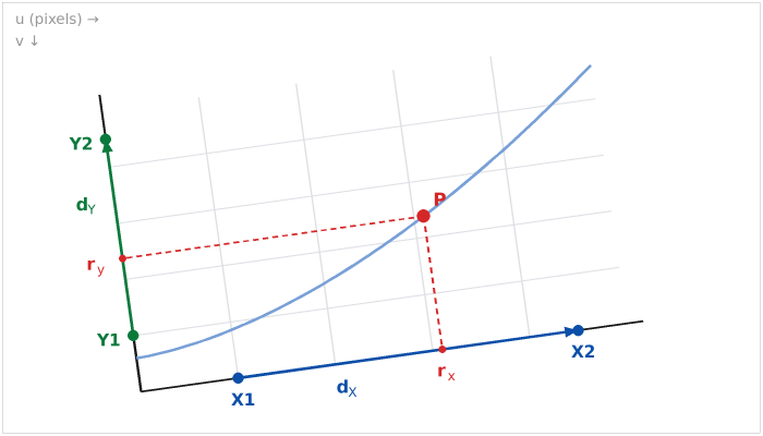
A scanned or photographed chart is seldom perfectly level, so the tool does not assume that the x axis runs along the pixel rows. It takes the direction of each axis from the two points you mark on it.
The equations
Positions in the picture are measured in pixels: u to the right and v downward from the top left corner (the usual convention for images). The four calibration points are X1 = (uX1, vX1), X2, Y1 and Y2, and the picked point is P = (up, vp).
dX = X2 − X1 = (dXu, dXv) and dY = Y2 − Y1 = (dYu, dYv)
are the directions of the two axes. The point P is reached from X1 by going some fraction rx of dX along the x axis and then some distance parallel to the y axis. Solving that pair of equations for rx, and the same from Y1 for ry, gives
Cxy = dXu dYv − dXv dYu
rx = [(up − uX1) dYv − (vp − vX1) dYu] / Cxy
ry = [dXu (vp − vY1) − dXv (up − uY1)] / Cxy
Cxy is the cross product of the two directions; it is zero only if the two axes are parallel, which the tool refuses. For a chart that sits level in the picture, dXv = 0 and dYu = 0 and the fractions reduce to rx = (up − uX1) / (uX2 − uX1) and ry = (vp − vY1) / (vY2 − vY1): plain proportion along each axis.
Linear axis. With X1 and X2 the values you typed for the two points,
x = X1 + rx (X2 − X1)
Logarithmic axis. On a log axis equal distances mean equal ratios: the distance from 1 to 10 is the distance from 10 to 100. The ruler is linear in the logarithm of the value, log x = log X1 + rx (log X2 − log X1), which is the same as
x = X1 (X2 / X1)rx
Halfway between the ticks 1 and 100 is therefore 10, not 50.5. The y axis is treated in the same way with ry, Y1 and Y2, and each axis may be linear or logarithmic independently. The result page writes these equations out with the numbers of your first point.
Square to the image (Advanced). With this choice dXv and dYu are set to zero: x is read from the pixel column alone and y from the pixel row alone. Use it when the chart is level and it is easier to mark the points anywhere than exactly on an axis.
Accuracy: what one pixel is worth
The result page states how much the value changes when a click moves by one pixel. On a linear axis that is the span between the calibration values divided by their distance in pixels; on a logarithmic axis it is a constant factor, so the percentage error is the same everywhere on the axis. A careful click is good to about one pixel, and the line of a printed curve is itself several pixels wide, so three significant figures are usually all a chart can give. Two things improve it: a larger picture (zoom the source before taking the screenshot) and calibration points far apart.
The five sample charts under "Try this" were drawn by a script from known formulas. The pixel positions stored with them give the formulas back to within one pixel (1.25 pixels for the crooked scan); the test of this tool checks that. A published check of a similar digitizing program, in which two people extracted 3,596 points from 36 graphs, reported high levels of agreement between the two coders and of validity (Drevon, Fursa and Malcolm, 2017).
Interpolation and resampling
If you ask for y at given x values, the points of each curve are sorted by x and y is read from the straight line between the two neighboring points. On a logarithmic axis the straight line is drawn in the logarithm, so that it is straight on the chart as printed. Nothing is extrapolated beyond the first and last point. Resampling tabulates the same interpolation at evenly spaced x values (evenly spaced in log x on a logarithmic x axis). The error of a straight line between points grows with the curvature and with the square of the spacing: click more points where the curve bends.
What it assumes
- The axes are straight and each scale is uniform: linear, or logarithmic, from end to end. Broken axes, date axes with months of unequal length, probability scales and polar or triangular charts are not covered.
- The picture is a flat, undistorted view of the chart. A turn, a different stretch in each direction and a shear are all handled exactly, because the calibration uses the direction of each axis. A photograph taken at an angle (perspective), a curled page or lens distortion is not.
- In the default mode, X1 and X2 lie on the x axis or on one grid line parallel to it, and Y1 and Y2 on the y axis or on one grid line parallel to it.
- The values you type for the calibration points are right. Everything else follows from them.
When it misleads
- The printed curve is not the data. A smooth line through scattered measurements, a curve drawn with a thick pen, or a figure redrawn by a publisher hides the scatter and may be off by more than a click.
- Markers that overlap or lie on top of a line are placed by eye. Use the magnifier and the arrow keys.
- A compressed picture (a small JPEG) smears edges by a few pixels. Use the largest, sharpest copy you can get.
- Interpolation between sparse points cuts corners: the straight line lies inside a curve that bows outward.
- The numbers are a reading, with the precision of a reading. Quote them to the figures the accuracy line supports, and cite the source of the chart.
Common mistakes
- Treating a log axis as linear. The replotted chart on the result page then bends where the original was straight. Check the tick labels: 1, 10, 100 is logarithmic.
- Interpolating a log scale by eye as if it were linear. Halfway between 10 and 100 on a log axis is 31.6, not 55.
- Calibration points too close together. A one-pixel error in a calibration point is magnified over the whole axis. Use the first and last labeled ticks.
- Typing the value of the wrong tick, or reading an axis label in thousands ("× 10³") as plain numbers.
- Forgetting that v runs downward. In pixels the top of the picture is v = 0, so a larger y value has a smaller v. The equations take care of it through the sign of dYv.
- Marking X1 and X2 at different heights on a level chart. The tool then reads the chart as turned. Put both on the axis line, or choose "Square to the image".
- Using a logarithmic axis with a zero. A log axis has no zero; a tick labeled 0 on such a chart is a drafting shortcut, and its value cannot be used for calibration.