Tools › Finance and Business › Finance › Engineering Economy Factors › Method
Engineering Economy Factors: Method
Open the Engineering Economy Factors tool
Engineering Economy Factors: Moving Money Through Time
The tool takes an interest rate and a short list of cash flows and tells you what they are worth as one amount now (P), one amount later (F) or the same amount every period (A), writing each step in the factor notation used in engineering economy courses and on the FE exam. It can also work backward: given the cash flows, it finds the interest rate, the number of periods or the one amount that makes them balance. An illustration of the method, not financial advice.
The idea: equivalence
Money has a time value: 1,000 today and 1,000 in five years are not the same thing, because 1,000 today can earn interest for five years. Two sets of cash flows are equivalent at an interest rate i when they have the same worth at any one point in time. Every problem in engineering economy is the same move: slide each cash flow along the time line to a common date, multiplying by a factor that depends only on i and on the number of periods n, then add.
The cash-flow diagram is the picture of the problem. Time runs to the right in whole periods; period 0 is now, and a cash flow "in period 3" arrives at the end of period 3. An arrow up is money received, an arrow down money paid. Draw it before touching a formula: most wrong answers come from a wrong n, and the diagram shows n.
The factors
The notation (X/Y, i, n) reads "find X given Y, at interest rate i per period, over n periods". With end-of-period cash flows and compounding once per period:
| Factor | Name | Formula | Use |
|---|---|---|---|
| (F/P, i, n) | single payment compound amount | (1 + i)n | F = P (F/P, i, n) |
| (P/F, i, n) | single payment present worth | (1 + i)−n | P = F (P/F, i, n) |
| (P/A, i, n) | uniform series present worth | [(1 + i)n − 1] / [i (1 + i)n] | P = A (P/A, i, n) |
| (A/P, i, n) | capital recovery | i (1 + i)n / [(1 + i)n − 1] | A = P (A/P, i, n): a loan payment |
| (F/A, i, n) | uniform series compound amount | [(1 + i)n − 1] / i | F = A (F/A, i, n): regular saving |
| (A/F, i, n) | sinking fund | i / [(1 + i)n − 1] | A = F (A/F, i, n): deposits to reach a goal |
| (P/G, i, n) | arithmetic gradient present worth | [(1 + i)n − i n − 1] / [i2 (1 + i)n] | P = G (P/G, i, n) |
| (A/G, i, n) | arithmetic gradient to uniform series | 1 / i − n / [(1 + i)n − 1] | A = G (A/G, i, n) |
All eight come from one fact, F = P (1 + i)n, and the sum of a geometric progression. At i = 0 they reduce to simple counting: (P/A) = (F/A) = n, (P/G) = n (n − 1) / 2, (A/G) = (n − 1) / 2. Pairs are reciprocals: (A/P) = 1 / (P/A), (A/F) = 1 / (F/A), (P/F) = 1 / (F/P); and (A/P) = (A/F) + i.
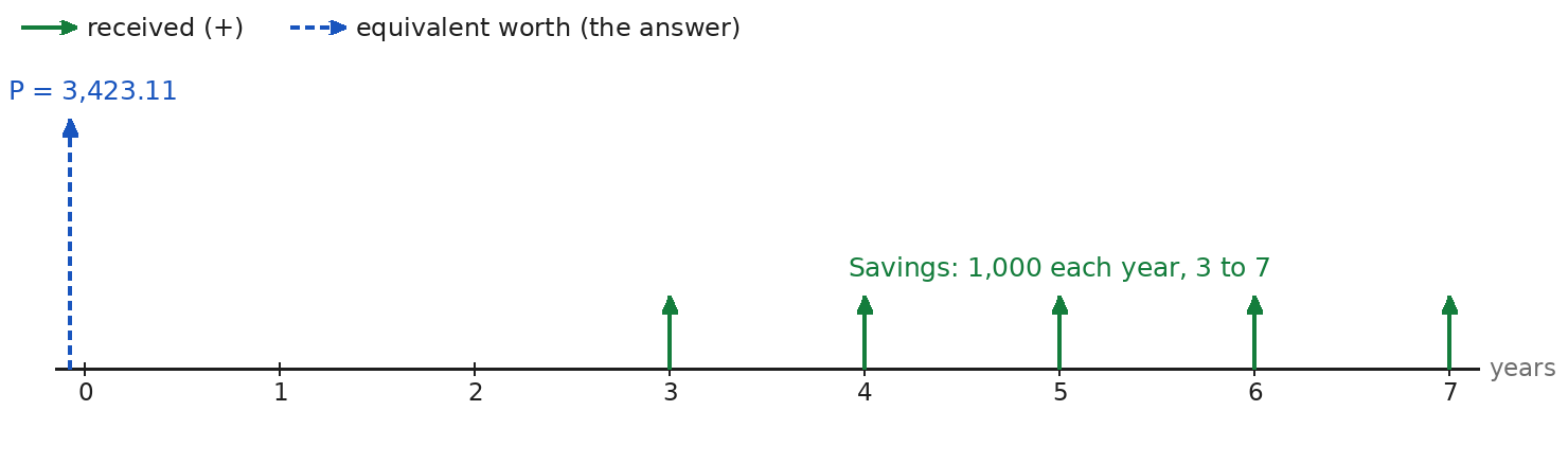
Where a series factor puts its answer. (P/A, i, n) gives the worth one period before the first amount of the series; (F/A, i, n) gives the worth at the last amount. A series that runs from period 3 to period 7 has n = 5 and its P/A answer sits at period 2, so one more factor, (P/F, i, 2), is needed to bring it to period 0 (Figure 1). A series whose first amount is at period 0 (rent or a lottery annuity paid in advance) has its P/A answer at period −1 and is moved forward with (F/P, i, 1).
Arithmetic gradient. A cash flow that changes by the same amount G each period (4,000, 4,500, 5,000, …) is split in two: a uniform series of the first amount, and a gradient series 0, G, 2G, …, (n − 1) G. The gradient factor is defined for that second series: nothing in the first period, G in the second. So P = A1 (P/A, i, n) + G (P/G, i, n), with n the number of periods of the whole series, and the answer one period before the first amount, exactly as for P/A.
Geometric gradient. A cash flow that grows by the same percentage g each period (A1, A1(1 + g), A1(1 + g)2, …) has the present worth, one period before the first amount, P = A1 [1 − ((1 + g) / (1 + i))n] / (i − g), and P = n A1 / (1 + i) when g = i. NIST Handbook 135 calls the same thing the modified uniform present value factor, written for a first amount of A0 (1 + e).
Nominal and effective interest
A rate quoted as "r per year, compounded m times a year" is a nominal rate: the rate actually applied each compounding period is r / m, and over a year it grows to the effective rate ia = (1 + r / m)m − 1. With continuous compounding ia = er − 1. A card at 24.99 % nominal compounded daily costs 28.38 % a year in effect. The factors need the rate per cash-flow period: when payments are monthly and compounding is monthly, i = r / 12; when the two differ, the tool uses i = (1 + ia)1 / p − 1 with p cash flows a year, the rate that gives the same effective yearly rate.
Solving for an unknown
Setting the present worth of all the cash flows to zero gives one equation, so one unknown can be found. For this the cash flows need both signs: what is paid against what is received.
An amount enters the present worth in proportion, so it is solved directly: X = −(worth of everything else) / (factor of its row). The loan payment A = P (A/P, i, n) and the sinking fund deposit A = F (A/F, i, n) are the two classic cases. The number of periods of a loan paid by a uniform amount has the closed form n = −ln(1 − P i / A) / ln(1 + i), which exists only when the payment A is larger than the first period's interest P i; the tool solves the general case numerically and reports the fractional n together with what it means in whole periods. The interest rate cannot be isolated from the factor formulas; it is found by trial (here by bisection between −99 % and 1,000 % per period). It is the internal rate of return of the cash flows. If the cash flows change sign more than once there can be more than one such rate, and the tool lists them all.
Comparing two alternatives
With equal lives, the alternative with the higher present worth (the lower present cost) at the chosen rate is the more economical. With unequal lives the present worths over each life are not comparable, since one buys more years of service than the other. Two standard repairs give the same ranking: compare the equivalent uniform worth per period, A = P (A/P, i, life); or compare present worths over the least common multiple of the lives, repeating each alternative as often as needed. Both rest on the same assumption: each alternative is replaced by an identical one at the same cost. The incremental rate of return is the rate at which the difference between the two sets of cash flows (dearer minus cheaper, over the common period) has zero present worth: if it exceeds the rate you require, the extra investment pays for itself. Comparing the two alternatives' own rates of return instead is a well-known error.
What it assumes
Cash flows fall at the end of whole periods, and period 0 is now. One interest rate holds for the whole time, for money owed and money held alike. Amounts are certain. The currency does not matter but must be the same throughout, and amounts and rate must both be in real terms or both in nominal terms. Taxes, depreciation and inflation are in the result only if they are in the numbers entered. The comparison of unequal lives assumes identical replacement.
When it misleads
When the timing is not end-of-period (monthly rent paid in advance entered as periods 1 to 12 instead of 0 to 11 shifts every amount by a month). When a nominal rate is used with yearly factors, or a yearly rate with monthly payments. When the horizon is very long: 60 guilders become hundreds of billions over 400 years at 6 %, but 46 billion at 5.25 %: small changes in the rate swamp everything else, and no rate is known for centuries. When an unknown rate is not unique. When the lives of two alternatives differ and replacement at the same cost is not realistic (prices and technology change): then choose a study period and estimate the salvage values at its end instead. A loan or card with fees, variable rates or minimum-payment rules is not the constant-rate loan computed here.
Common mistakes in hand solutions
- Wrong n for a shifted series. A series from period 3 to period 7 has 7 − 3 + 1 = 5 amounts, not 4 and not 7.
- Forgetting where P/A lands. The answer of (P/A, i, n) is one period before the first amount, not at period 0 and not at the first amount. Discount it the remaining periods with (P/F, i, first − 1).
- Using n − 1 in the gradient factor. (P/G, i, n) takes the n of the whole series although the gradient series has only n − 1 non-zero amounts; the zero in the first period is built into the factor.
- Dropping the uniform part of a gradient. 4,000, 4,500, 5,000 is A = 4,000 plus G = 500, not G alone.
- Mixing a decreasing gradient's signs. Costs entered as negative amounts that rise each year need a negative G as well.
- Dividing a yearly effective rate by 12. Only a nominal rate compounded monthly is divided by 12. From an effective yearly rate the monthly rate is (1 + ia)1/12 − 1.
- Using the nominal rate in yearly factors. 12 % compounded monthly with yearly cash flows needs i = 12.68 %, not 12 %.
- Placing F/A's answer a period late. (F/A, i, n) gives the worth at the moment of the last deposit, which earns no interest.
- Adding amounts at different dates. Cash flows may be added only after they have been moved to the same period.
- Losing the sign. In an equation of worth = 0 the amounts paid and received carry opposite signs; a salvage value is a receipt at the end, not a cost.
- Comparing present worths over unequal lives, or choosing between alternatives by their separate rates of return instead of the rate on the difference.
- Linear interpolation in a factor table over a wide gap. Factors are curved in i and in n; compute them from the formula instead (the tool's table is computed for your exact rate).
Checks
The single-payment and uniform-series factors reproduce every printed value of Tables 3-1 and 3-2 of NIST Handbook 135 (2020) at 3.0, 1.3 and 1.5 percent and its worked examples (862.61; 457.97; the geometric factor 4.8562; 614, 825, 9,010, 1,276 and 130 of its Chapter 17). The gradient factors, the worth of mixed cash flows, the solved rates, amounts and numbers of periods and the unequal-life comparison are checked against period-by-period sums computed independently with numpy and scipy. No printed table of gradient factors from an open source was found; those rest on the summation check alone.