Tools › Finance and Business › Auditing › Audit Sampling › Method
Audit Sampling: Method
Method: the Estimators and Their Standard Errors, the Stringer Bound, the Random Number Generator, What It Assumes and Common Mistakes
What the tool does
An auditor who cannot examine every item examines a random sample and carries what it shows to the whole population. The tool does the three pieces of arithmetic that this takes: it sizes a sample, draws it from a pasted list with a seeded random number generator so that anyone can draw it again, and projects the errors found in the sample to the population with a statement of how far off the projection may be.
It does this in two families. Classical variables sampling treats every item alike and estimates the total error with a two-sided confidence interval, as the RAT-STATS program of the U.S. Department of Health and Human Services, Office of Inspector General does. Monetary unit sampling treats every dollar alike, so large items are more likely to be drawn, and gives an upper limit on overstatement.
The idea: a sample mean, scaled up, with a margin
Let the population hold N items, of which n are sampled. For each sampled item the error is d = book amount − audited amount, so an overpayment is positive. The difference estimator of the population error is the mean sampled error times the number of items:
E = N · d̄ standard error SE = N · sd · √[(N − n) / (N · n)]
where sd is the standard deviation of the sampled errors (divisor n − 1) and the root holds the finite population correction: a sample that is a large part of the population leaves less to guess. The two-sided confidence interval is
E ± t · SE (one stratum: Student's t with n − 1 degrees of freedom)
The half-width t · SE is the precision amount; as a percentage of E it is the precision percent.
Stratified samples
When the population is split into strata (for example by size of claim) and a random sample is drawn in each, the estimates and the variances of the strata add:
E = Σ Nh · d̄h SE² = Σ Nh² · (1 − nh / Nh) · sh² / nh
The limits of the stratified total use the normal Z-value (1.2816, 1.6449 and 1.9600 for 80, 90 and 95 %), and each stratum alone uses t, as RAT-STATS does. A stratum examined in full (nh = Nh) adds its exact error and no variance.
Three estimators on one sample
- Difference: as above. It is the RAT-STATS appraisal of the difference values and needs no book total.
- Mean per unit: the same formulas applied to the audited amounts give an estimate A of the audited total; the error is the book total X less A. Its standard error follows the spread of the amounts themselves, which is usually far larger than the spread of the errors.
- Ratio: R = Σ Nh d̄h / Σ Nh x̄h is the error per book dollar in the sample (x is the book amount), and E = R · X. Its variance uses the spread of d − R · x, so it is small when errors are proportional to book amounts. This is the combined ratio estimator of survey sampling; it is slightly biased in small samples and is not one of the RAT-STATS variable appraisals.
The estimator is chosen in the sampling plan, before the results are seen. Choosing the one with the most favorable interval afterward makes the stated confidence untrue.
One-sided and two-sided
A limit of a two-sided interval is also the limit of a one-sided interval with half the risk. The lower limit of a two-sided 80 % interval is the lower limit of a one-sided 90 % interval, which is the figure the Medicare Program Integrity Manual names in section 8.4.5; the lower limit of a two-sided 90 % interval is that of a one-sided 95 % interval. The tool tabulates the two-sided 80, 90 and 95 % limits, as RAT-STATS prints them.
Sample size for a precision target
For a precision amount P = (precision percent) × (expected total), RAT-STATS sizes an unrestricted sample as
n = (σ · N)² / [(P / Z)² + N · σ²]
and a stratified one as n = (Σ Nh σh)² / [(P / Z)² + Σ Nh σh²], shared among the strata in proportion to Nh σh. The spread σ of the errors is not known before the audit; from an expected error rate p the program assumes that an item in error is wholly in error and that such items look like the book amounts (mean μ, standard deviation σR), which gives a mean error of p · μ and σ = √(p · [σR² + (1 − p) · μ²]). The tool takes μ and σR from the pasted population, stratum by stratum. If a stratum's share reaches all of its items, it is examined in full and the formula is applied again to the others, so that the target is still met.
Monetary unit sampling
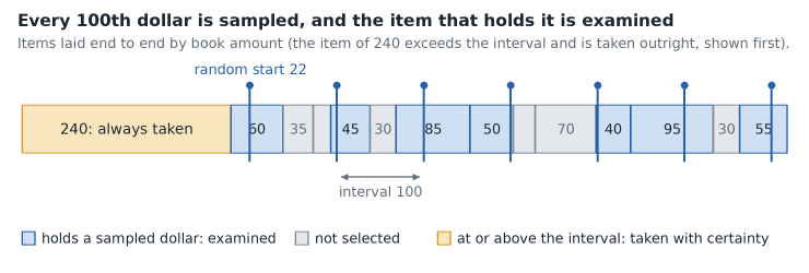
The population is seen as a row of dollars. With a sampling interval J = book value / n, one dollar in every J is sampled after a random start, and the item that holds it is examined. An item of J or more is always taken. If a sampled item with book amount b is found to be worth a, its tainting is t = (b − a) / b, and the sampled dollar is taken to be misstated by that share.
The Stringer bound on the overstatement of the population, with the taintings ranked from largest to smallest (t1 ≥ t2 ≥ …), is
upper limit = J · F0 + J · Σ ti + J · Σ (Fi − Fi−1 − 1) · ti
The three terms are the basic precision, the projected misstatement and the incremental allowance. Fi is the Poisson confidence factor: the mean number of errors for which seeing i or fewer has a probability of one minus the confidence level. F0 = −ln(1 − confidence), which is 3.00 at 95 % and 2.30 at 90 %; in general Fi is half the chi-square quantile with 2(i + 1) degrees of freedom. The tool computes the factors from the gamma distribution and uses no published table. Errors in items taken with certainty are known exactly and are added as they are.
Why the limit is not zero when no error is found. A clean sample of n dollars does not show that every dollar is right. If a share q of the dollars were misstated, the chance that all n sampled dollars are clean is about e−nq. That chance falls to 5 % only when n · q = 3.00, so at 95 % confidence a misstatement of up to 3.00 × J cannot be ruled out.
Sample size. The tool finds the smallest n for which the upper limit would stay within the tolerable misstatement TM if exactly the expected misstatement EM were found: F(n · EM / BV) / n ≤ TM / BV, where the factor F is carried to a fractional number of errors by the gamma distribution. With EM = 0 this is n = F0 · BV / TM.
The random numbers
A selection that cannot be drawn again cannot be checked, so the generator is fixed and written out here. The seed s (a whole number from 1 to 2,147,483,646) is first scrambled by the 32-bit finalizer of MurmurHash3, with all arithmetic modulo 232:
h = s; h ^= h >> 16; h *= 0x85EBCA6B; h ^= h >> 13; h *= 0xC2B2AE35; h ^= h >> 16; x0 = 1 + (h mod 2,147,483,646)
and the numbers then come from the Lehmer generator of Park and Miller with the multiplier 48,271:
xk+1 = 48,271 · xk mod 2,147,483,647 uk = xk / 2,147,483,647 (u1 is the first number used)
Check values: the scrambler turns 1 into 0x514E28B7; seed 2026 gives x0 = 1,504,179,461 and u1 = 0.849672063.
- Classical sample: every line of the population, in pasted order, receives the next number; within each stratum the items with the smallest numbers are the sample.
- Monetary unit sample: the first sampled dollar is u1 · J into the running total of the items below the interval, in pasted order, and the others follow every J.
The same seed, the same lines and the same order give the same sample. Record all three with the working papers. RAT-STATS has a random number generator of its own, so a seed used in that program does not draw the same sample here.
Pasted rows
One item per line. Columns are separated by a tab, a comma or a semicolon, or by spaces when a line has none of these. Population: id, book amount and an optional stratum. Sample: id, book amount, audited amount and an optional stratum. Population summary: stratum, count and book total. One header line is allowed. Amounts are plain numbers without thousands separators. Each box takes 10,000 rows.
What it assumes
- The sample is a probability sample of the population that the summary describes: simple random within each stratum for the classical family, proportional to size for monetary unit sampling. The arithmetic cannot tell whether it was.
- The classical intervals rest on the central limit theorem: the sample mean is taken as normally distributed. This holds well for large samples of well-behaved errors.
- The audited amount of each sampled item is right. A wrong audit finding is projected like any other.
- For monetary unit sampling, no item is overstated by more than its book amount (tainting at most 100 %), and book amounts are positive.
When it misleads
- Few errors, or a few large ones. When most sampled items have no error and a handful have large ones, the errors are far from normal and the classical interval can cover the truth less often than its label says. Monetary unit sampling was designed for populations with few errors.
- No errors in a classical sample. Every difference is zero, so the standard error is zero and the interval has no width. That is what the formula returns; it is not evidence that the population is free of error.
- Understatements in a monetary unit sample. The Stringer bound is a bound on overstatement. The tool reports understatements and their projection beside it and does not net them into the limit.
- The Stringer bound is cautious. In published simulation studies its true confidence has been at or above the stated level, often well above it when errors are found, although no general proof of this exists. The limit can therefore be larger than a tighter method would give.
- A plan is a forecast. The sample size comes from an assumed error rate and an assumed shape of the errors. The precision achieved is known only after the audit.
- Missing items. Zero and negative book amounts cannot be drawn by a monetary unit sample; the tool sets them aside and says so.
Common mistakes
- Multiplying the error rate of the sample by the book total. A share of items in error is not a share of dollars in error, unless every error is 100 % of its item.
- Projecting a stratified sample as if it were one random sample. Each stratum is scaled by its own Nh / nh.
- Leaving out the finite population correction when the sample is a large part of the population, or applying it twice.
- Using n in place of n − 1 in the standard deviation.
- Reading a two-sided 90 % lower limit as a one-sided 90 % limit. It is a one-sided 95 % limit.
- In monetary unit sampling, projecting the dollar error of an item in place of its tainting, or projecting the error of an item that was taken with certainty.
- Changing the order of the population file after the draw. The selection depends on the order of the lines.
- Replacing an awkward sampled item with a convenient one. The sample is then no longer random and none of the formulas apply.
Scope
The tool computes. Whether a sample design is valid for a given audit, what confidence level and estimator a program or contract calls for, and what follows from a projected amount are matters of the auditor's judgment and of the rules that govern the audit. A projected amount is a reason to look, not a finding. Cluster and multistage designs, attribute sampling for error rates, and the cell and bootstrap variants of monetary unit evaluation are not covered. For digit tests on the same pasted amounts see Benford's Law Test; for lot acceptance by attributes see Acceptance Sampling.