Round Hole Uniaxial Stress: Method

Round Hole in an Infinite Plate under Uni-axial Load: the Kirsch Solution

Problem Statement

A large, thin, flat plate contains a circular hole of diameter D (radius a = D/2) and carries a uniform uni-axial stress σ_x far from the hole. The plate is linear elastic, isotropic and in plane stress, and it is "infinite": every edge is far enough from the hole that it does not disturb the stress field (in practice, a plate width and length of more than about 10 hole diameters, with the hole at least 5 diameters from any edge). The question is the state of stress at a point P near the hole, given by its distance r from the hole center and the angle θ between the radius to P and the load axis.

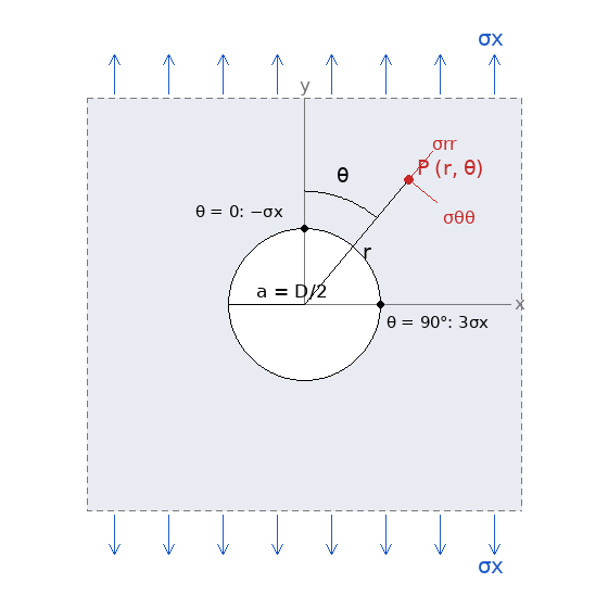
Figure A: Convention used by the tool. The load σ_x acts along the vertical y axis; θ is measured from that axis to the radius through P; σ_rr acts along the radius and σ_θθ across it.

Key Assumptions

Infinite plate, linear elastic, plane stress, uni-axial load. The plate edges are far from the hole; the material is isotropic and stays elastic (no yielding at the 3σ_x peak); the plate is thin enough that through-thickness stresses are negligible; the hole is open (no fastener or pin) and traction-free. The solution does not depend on the elastic constants, so the stresses are the same for every isotropic material.

Solution

Kirsch (1898) solved the problem with an Airy stress function in polar coordinates. The uniform far-field stress is split into a hydrostatic part σ_x/2, which the hole disturbs through the axisymmetric terms, and a pure-shear part (σ_x/2) cos 2θ, which the hole disturbs through the cos 2θ terms. The stress function

Φ = (σ_x/4) (r² − 2a² ln r) − (σ_x/4) (r² − 2a² + a⁴/r²) cos 2θ

satisfies the biharmonic equation, gives the uniform stress at r → ∞, and makes the hole edge traction-free (σ_rr = σ_rθ = 0 at r = a). Differentiating it gives the stresses the tool evaluates:

σ_rr = (σ_x/2) (1 − a²/r²) + (σ_x/2) (1 − 4a²/r² + 3a⁴/r⁴) cos 2θ

σ_θθ = (σ_x/2) (1 + a²/r²) − (σ_x/2) (1 + 3a⁴/r⁴) cos 2θ

σ_rθ = −(σ_x/2) (1 + 2a²/r² − 3a⁴/r⁴) sin 2θ

The tool writes the radial and shear coefficients in factored form, (1 − a²/r²)(1 − 3a²/r²) and (1 − a²/r²)(1 + 3a²/r²), which multiply out to the expressions above and show at a glance that both vanish on the hole edge. This is Kirsch's own notation: page 799 of the 1898 paper prints the equations in exactly this form, with the angle measured from the load axis and the load drawn vertical in his Fig. 5, which is the convention of Figure A.

Hole Edge and Stress Concentration Factor

On the free edge r = a only the tangential stress survives:

σ_θθ(a, θ) = σ_x (1 − 2 cos 2θ)

• θ = 90° and 270° (the sides of the hole, on the axis normal to the load): σ_θθ = 3σ_x. This is the maximum stress in the plate, so the stress concentration factor of a round hole in an infinite plate is K_t = 3, independent of the hole size and of the material.
• θ = 0 and 180° (the top and bottom of the hole, on the load axis): σ_θθ = −σ_x. A tensile load puts the top and bottom of the hole into compression of the same magnitude as the applied stress.
• The tangential stress changes sign where cos 2θ = 1/2, i.e. at θ = 30° from the load axis.

The disturbance decays quickly: along the axis normal to the load, σ_θθ/σ_x = 1 + a²/(2r²) + 3a⁴/(2r⁴), which is 1.22 at r = 2a and 1.07 at r = 3a. That is why a hole can be treated as "in an infinite plate" when the edges are a few diameters away.

Principal Stresses at the Probed Point

Away from the edge all three polar components are non-zero, and the tool transforms them to principal values with the plane-stress relations:

σ_max, σ_min = (σ_rr + σ_θθ)/2 ± √[((σ_rr − σ_θθ)/2)² + σ_rθ²]

τ_max = √[((σ_rr − σ_θθ)/2)² + σ_rθ²] = (σ_max − σ_min)/2

tan 2φ_p = 2σ_rθ / (σ_rr − σ_θθ)

φ_p is measured from the radial direction. The arctangent gives two directions 90° apart, one for each principal stress; the tool picks the one belonging to σ_max (when σ_θθ > σ_rr the arctangent branch locates σ_min, so 90° is added) and keeps it within ±90°. φ_x = φ_p + θ gives the same direction from the load axis. On the hole edge, where σ_rr = σ_rθ = 0, the principal directions are simply radial and tangential. The in-plane τ_max is the quantity to compare with a shear allowable; the absolute maximum shear stress, which includes the out-of-plane direction, is σ_max/2 when both in-plane principal stresses are positive.

Reading the Plots

• σ_θθ fringe. Shows the Kirsch component the equations compute. The 3σ_x lobes at the sides and the −σ_x spots at the top and bottom are real; the X-shaped pattern far from the hole is not a stress concentration but the far-field value σ_θθ → σ_x sin²θ, which is just the uniform stress resolved onto a rotating direction.
• σ_max fringe. Shows stress severity. The far field is uniform σ_x, the lobes are the same, the top and bottom of the hole read zero because the compression there is σ_min, and the cyan "stress shadow" above and below the hole is where the load flows around the hole and σ_max drops below σ_x.
• Line plots. The edge curve σ_x(1 − 2 cos 2θ) and the decay along the two axes; the user input point is marked where it lies on the plotted line.

Limits of the Solution

• Finite width. When the plate width W is not large compared with D, the net-section stress rises and K_t based on the gross stress falls below 3 while K_t based on the net stress rises above it. Howland (1930) solved the strip; Heywood's fit K_t,net = 2 + (1 − D/W)³ is the usual design form and the charts in Peterson's Stress Concentration Factors cover D/W up to 0.6. This tool does not apply a finite-width correction.
• Biaxial load. The solution is linear, so a second remote stress is handled by superposition: equal biaxial tension gives K_t = 2, pure shear (equal and opposite stresses) gives K_t = 4.
• Yielding. A 3σ_x peak reaches the yield strength at σ_x = F_ty/3; beyond that the elastic solution overstates the peak stress and a Neuber or Glinka estimate is needed.
• Loaded holes (pins, fasteners) have a different field; see the fastened-joint tools.