Round Hole General Load: Method

Round Hole in an Infinite Plate under General In-plane Load

Problem Statement

A large, thin, flat plate with a round hole of diameter D (radius a = D/2) carries a uniform in-plane membrane state far from the hole, given as the stress resultants N_xx, N_yy, N_xy (force per unit width) and the plate thickness t. The far-field stresses are σ_xx^∞ = N_xx/t, σ_yy^∞ = N_yy/t, τ_xy^∞ = N_xy/t. The plate is linear elastic, isotropic, in plane stress and infinite (edges far from the hole). The question is the stress at a point P(r, θ), θ measured from the y axis towards x, and the extremes on the hole edge.

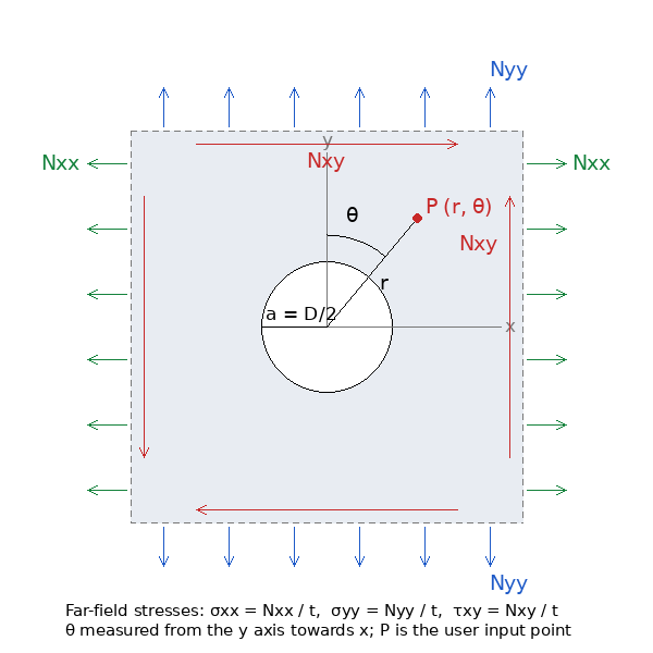
Figure A: Convention. N_xx and N_yy are positive in tension; N_xy is positive when it acts in +x on the top (+y) edge; θ is measured from the y axis towards x, the same convention as the uni-axial tools, where y is the load axis.

Key Assumptions

Infinite plate, linear elastic, plane stress, uniform far field. The resultants are uniform and the plate thin, so N/t is a uniform membrane stress with no bending. The hole is open and traction-free. The material stays elastic at the peak. The solution does not depend on the elastic constants.

Solution by Superposition

The Kirsch solution is linear in the remote stress. Resolve the far-field state into its principal values and direction,

S_1,2 = (σ_xx^∞ + σ_yy^∞)/2 ± √[((σ_xx^∞ − σ_yy^∞)/2)² + (τ_xy^∞)²],    tan 2φ = 2τ_xy^∞ / (σ_xx^∞ − σ_yy^∞),

and add the uni-axial Kirsch fields for S₁ and S₂. Written directly in the plate axes, with q = a²/r², the mean stress S_m = (σ_xx^∞ + σ_yy^∞)/2 and the deviatoric terms resolved on the radius at θ,

D(θ) = −(σ_xx^∞ − σ_yy^∞)/2 · cos 2θ + τ_xy^∞ sin 2θ,    E(θ) = (σ_xx^∞ − σ_yy^∞)/2 · sin 2θ + τ_xy^∞ cos 2θ,

the stresses are

σ_rr = S_m (1 − q) + D(θ) (1 − 4q + 3q²)

σ_θθ = S_m (1 + q) − D(θ) (1 + 3q²)

σ_rθ = E(θ) (1 + 2q − 3q²)

The signs follow the tool's convention (θ from y towards x, tangential direction in the sense of increasing θ). With σ_yy^∞ = σ_x and the other two zero, D = (σ_x/2) cos 2θ, E = −(σ_x/2) sin 2θ, and the equations reduce to those of the uni-axial tool. The tool checks its plots, which use the superposed complex-potential field of the elliptic tool with a = b, against these closed forms.

Hole Edge and Stress Concentration Factor

On the edge q = 1 and only the hoop stress remains: σ_θθ(a, θ) = (σ_xx^∞ + σ_yy^∞) − 4D(θ). Since D swings between ±(S₁ − S₂)/2, the extremes are

• σ_edge,max = 3S₁ − S₂, at the two points where the S₂ axis meets the hole (perpendicular to S₁);
• σ_edge,min = 3S₂ − S₁, at the two points on the S₁ axis.

Reference for K_t. There is no single applied stress, so the tool refers K_t to the maximum far-field principal stress: K_t = σ_edge,max/S₁ = 3 − S₂/S₁. Uni-axial: 3. Equal biaxial tension: 2 (the hoop stress is 2S all round). Pure shear (S₂ = −S₁ = −τ): 4, at 45° to the shear axes. Biaxial tension lowers the peak; a compressive S₂ raises it. When the far field has no tensile principal stress (S₁ ≤ 0) the ratios are formed with S₂ instead, so that the governing compressive peak is compared with the governing far-field compression.

Principal Stresses at the Probed Point

From σ_rr, σ_θθ, σ_rθ the tool gives σ_max, σ_min, τ_max and the direction of σ_max both from the y axis (φ_x) and from the radial direction (φ_p), each within ±90°. The direction of S₁ is reported in the same way (φ₁, from the y axis).

Reading the Plots

• σ_θθ fringe. The tangential stress about the hole center; on the edge it is the hoop stress, whose extremes sit on the far-field principal axes rather than on x and y. The color scale spans those two extremes in units of the reference stress.
• σ_max fringe. The maximum principal stress, uniform S₁ far from the hole.
• Line plots. The hoop stress around the edge versus θ, and the stresses along the x and y axes versus r/a. Under a general load these axes are not the principal axes, so the edge extremes appear in Figure 3 but not necessarily at the start of Figures 4 and 5.

Limits

• Finite width and yielding: as for the uni-axial tool; no finite-width correction is applied, and the elastic peak is valid up to σ_edge,max = F_ty.
• Bending (M_xx, M_yy, M_xy) is a different problem (Goodier, Reissner); only membrane resultants are handled here.