Round Hole Finite Strip: Method

Round Hole in a Finite-Width Strip under Tension (Howland's Series)

Problem Statement

A long, thin strip of width W and thickness t has a round hole of diameter D (radius a = D/2) on its center line and carries an axial load P. Far from the hole the stress is uniform, σ_g = P/(W t), the gross stress; across the hole the ligament of width W − D carries the same load at the mean net-section stress σ_n = P/((W − D) t). The strip is linear elastic, isotropic, in plane stress and long compared with its width. The questions are the stress at a point P(r, θ), θ measured from the load axis y towards x, the peak hoop stress on the hole and the factors K_tg = σ_max/σ_g and K_tn = σ_max/σ_n.

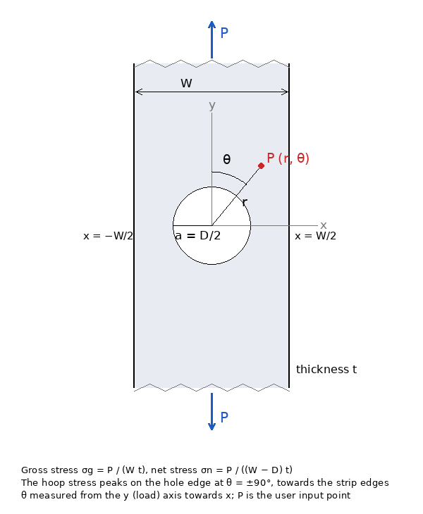
Figure A: Convention. The strip edges are at x = ±W/2, the load acts along y, and θ is measured from the y axis towards x, the same convention as the infinite-plate tools. The hoop stress peaks at θ = ±90°, the points of the hole nearest the strip edges.

Key Assumptions

Infinitely long strip, linear elastic, plane stress, central hole, axial load. The load is a uniform tension far from the hole; the strip edges and the hole are traction-free. Plates of finite length behave like the strip once their length exceeds about twice the width (Deghboudj et al. 2016). The solution does not depend on the elastic constants and is the same in plane strain. The material stays elastic at the peak. The series is carried to convergence for 0 < D/W ≤ 0.9.

Howland's Solution

Kirsch's solution for the infinite plate leaves tractions on the lines x = ±W/2; Howland (1930) removed them with an Airy stress function built from two families. With the handbook axes (tension along the strip axis ξ, edges at η = ±b, b = W/2) the function is

χ = σ_g η²/2 + ∑_j c_j [ F_j(r, θ) + E_j(ξ, η) ],

where the hole functions F_j are the Michell functions even in both axes and decaying with distance, ln r, r^−2m cos 2mθ and r^2−2m sin θ sin(2m − 1)θ, m = 1, 2, … Each has an exact Fourier-integral representation on the edges, e.g.

r^−2m cos 2mθ = (−1)^m/(2m − 1)! ∫₀^∞ α^2m−1 e^−αη cos αξ dα,

so the tractions it leaves on η = ±b are a cosine integral in ξ. The companion edge function

E_j = ∫₀^∞ [ C_j(α) cosh αη + D_j(α) αη sinh αη ] cos αξ dα

is also biharmonic and even, and its two coefficients are chosen mode by mode so that σ_ηη and τ_ξη vanish on the edges exactly (the denominator sinh 2αb + 2αb appears here). Every pair F_j + E_j therefore satisfies the edge conditions and decays along the strip, and equilibrium is automatic because every edge spectrum vanishes at α = 0. What remains is the traction-free hole: Howland re-expanded the edge functions about the hole in powers of r and solved the resulting infinite linear system for the c_j by successive approximation, by hand, for 2a/W up to 0.5.

The tool solves the same system numerically. The α-integrals are evaluated by Gauss–Legendre quadrature (200 nodes on [0, 60/b]; the integrands behave like α^k e^−2αb), and the 2N + 1 coefficients follow from the conditions σ_r = τ_rθ = 0 at 12N + 40 points of the hole edge by least squares, with N = 12 to 24 pairs depending on D/W. The residual traction on the hole is printed on the page; it is 10⁻¹³ σ_g for D/W ≤ 0.5 and 10⁻⁸ at 0.9, and the result does not change when the number of terms or quadrature nodes is doubled.

Stress Concentration Factors

The hoop stress on the hole is largest at θ = ±90°, the points nearest the strip edges, and most compressive on the load axis. The tool reports the gross factor K_tg = σ_max/σ_g, which grows without bound as the ligament narrows, and the net factor K_tn = σ_max/σ_n = K_tg(1 − D/W), which falls from the Kirsch value 3 towards 2 as D/W → 1. It also gives the stress at the strip edge on the net section, x = W/2, which is below σ_n: the ligament stress is highest at the hole and falls towards the free edge, while its integral over the ligament equals the load.

D/W	Ktg series	Ktn series	Howland fit (Peterson)	Finite element (2016)	Heywood Ktn
0.1	3.036	2.733	3.035	2.981*	2.729
0.2	3.153	2.522	3.148	3.156	2.512
0.3	3.374	2.362	3.367	3.391	2.343
0.4	3.747	2.248	3.732	3.771	2.216
0.5	4.348	2.174	4.314	4.366	2.125
0.6	5.318	2.127	5.255	5.344	2.064
0.7	6.987	2.096	6.889	7.020	2.027
0.8	10.350	2.070	10.216	10.39	2.008
0.9	20.416	2.042	20.237	20.5	2.001

Table 1: K_tg from the converged series against the expression fitted to Howland's table (Pilkey & Pilkey 2008) and the finite element values of Deghboudj et al. (2016, plate length twice the width); Heywood's K_tn = 2 + (1 − D/W)³. The series lies between the two at every ratio: 0 to 1.4 % above the fit to Howland's hand-computed values and 0.1 to 0.6 % below the finite element results. *The finite element value at 0.1 is below the Kirsch limit and reflects the mesh.

Checks

• As D/W → 0 the series gives K_tg → 3.00 (3.0014 at D/W = 0.02), the Kirsch value, and the hoop stress on the load axis → −σ_g.
• The stress σ_yy integrated across the ligament equals σ_g W/2 per half strip to 10⁻⁶ (equilibrium), and the field returns to the uniform gross stress along the strip as e^{−2.1 y/b}, the Papkovich–Fadle decay rate of a strip.
• The strip edges are traction-free to 10⁻¹⁶ σ_g at every point (exact by construction), the hole to the printed residual.

Limitations

• Central hole only; an eccentric hole or a hole near one edge is a different problem (Isida; Peterson Chart 4.2).
• D/W ≤ 0.9: for narrower ligaments the hole series converges too slowly (the number of terms is already raised to 24 above 0.8).
• Two-dimensional plane stress: through-thickness variation of the peak (Sternberg & Sadowsky; Pilkey Chart 4.1 notes) is not represented.
• The tool draws the stress field within four hole radii or, for wider holes, across the whole strip width; for D/W < 0.29 the strip edges lie outside the window.