Elliptic Inclusion: Method

Elliptic Inclusion in an Infinite Plate under General In-plane Load

Problem Statement

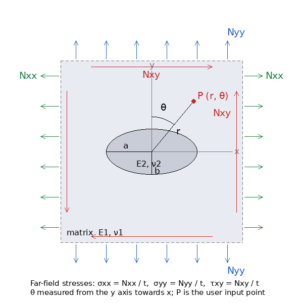
A large thin plate (matrix E₁, ν₁) contains an elliptic inclusion with semi-axes a and b, its a axis inclined by β from the x axis, made of another material (E₂, ν₂) and perfectly bonded. The plate carries the uniform far-field state N_xx, N_yy, N_xy over the thickness t. Wanted are the uniform stress inside the inclusion, the stress at a point in either region, and the interface stresses governing matrix cracking, debonding and slip. The rigid inclusion and the empty (Inglis) hole are the limits; a = b is the circular inclusion.

Key Assumptions

Infinite plate, linear elastic isotropic materials, perfect bonding, plane stress or plane strain, aspect ratio between 0.2 and 5. No slip, separation, interference or thermal mismatch (an eigenstrain mismatch adds an Eshelby solution that can be superposed). The series solution is truncated to a relative accuracy near 10⁻⁸; for aspect ratios beyond 5 the number of terms grows and the tool declines the input.

Solution

The exterior of the unit circle is mapped onto the matrix by z = ω(ζ) = R(ζ + m/ζ), R = (a + b)/2, m = (a − b)/(a + b), as in the elliptic-hole tools. By Eshelby's theorem the stress inside the inclusion is uniform, so its potentials are φ₂ = Dz, ψ₂ = Fz. The matrix potentials are φ₁(ζ) = ΓRζ + Σα_kζ^−k and ψ₁(ζ) = Γ′Rζ + Σβ_kζ^−k, where Γ = (σ_xx^∞ + σ_yy^∞)/4 and Γ′ = [(σ_yy^∞ − σ_xx^∞) + 2iτ_xy^∞]/2 in the inclusion's frame. Unlike the circle, for which only ζ⁻¹ and ζ⁻³ appear, the mapping's poles at ζ = ±√m make these series infinite, with terms decaying like |m|^k (Hardiman gives them in closed form through the mapping). The tool keeps as many terms as needed for |m|^k < 10⁻⁹ and determines all coefficients, with D and F, from the continuity of traction, φ + zφ̄′ + ψ̄, and of displacement, (κφ − zφ̄′ − ψ̄)/2μ, imposed at four points per term around the interface and solved in the least-squares sense; the collocation residual is reported and is at rounding level. The stresses follow from σ_xx + σ_yy = 4 Re Φ, σ_yy − σ_xx + 2iτ_xy = 2[z̄Φ′ + ψ′]/ω′.

Checks built into the development: a = b reproduces the circular-inclusion solution to 14 digits; E₂ = 0 reproduces the Inglis hole (error 6×10⁻⁶ ksi on 750 ksi at a/b = 2, 4×10⁻⁹ at a/b = 4, converging geometrically with the number of terms); matched materials give the far field everywhere; for an elastic inclusion the interface normal and shear stresses and both displacement components are continuous across the bond while the tangential stress jumps; for a rigid inclusion the matrix displacement on the interface vanishes.

Interface Stresses and Concentration Factors

As for the circular inclusion the tool scans the interface on the matrix side and reports the tangential (hoop), normal (debonding) and shear extremes with the polar angle of each point, referred to the maximum far-field principal stress S₁: K_hoop, K_rad and K_I = σ_{max,inclusion}/S₁. A stiff inclusion elongated across the load attracts load like a short fiber and raises the debonding stress at its ends; a soft one elongated across the load approaches the elliptic hole, whose matrix factor is 1 + 2a/b.

Limits

• Imperfect bonding and eigenstrains (thermal or transformation mismatch) are not included.
• Aspect ratios beyond 5 (fibers, platelets) need many terms; the slender limit is the crack or the rigid line inclusion.
• Finite width and yielding: as for the hole tools.