Elliptic Hole Uniaxial Stress: Method

Elliptic Hole in an Infinite Plate under Uni-axial Load: the Inglis Solution

Problem Statement

A large, thin, flat plate contains an elliptic hole with semi-axis a across the load and semi-axis b along it, and carries a uniform uni-axial stress σ_x far from the hole. The plate is linear elastic, isotropic and in plane stress, and "infinite": every edge is far enough from the hole not to disturb the stress field. The question is the state of stress at a point P, given by its distance r from the hole center and the angle θ between that radius and the load axis, and the stress concentration at the hole edge. With a = b the hole is round and everything reduces to the Kirsch solution of the companion tool.

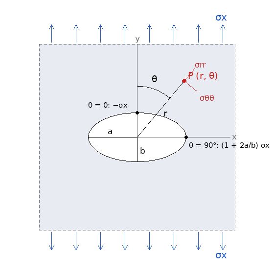
Figure A: Convention used by the tool. The load σ_x acts along the vertical y axis; a is the semi-axis across the load (along x), b the semi-axis along the load; θ is measured from the load axis to the radius through P.

Inclined hole. The input β rotates the hole: it is the angle of the semi-axis a from the horizontal, positive counterclockwise towards the load axis, so Figure A shows β = 0 and β = 90° puts a along the load (the same as swapping a and b). The probe angle θ is always measured from the load axis in the plate frame, not from the hole's axes.

Key Assumptions

Infinite plate, linear elastic, plane stress, uni-axial load. The hole may be aligned with the load or inclined to it by β; an inclined hole has an unsymmetric field whose edge extremes the tool finds by scanning the edge. The material stays elastic at the peak, the plate is thin, and the hole is open and traction-free. The solution does not depend on the elastic constants.

Solution

Inglis (1913) solved the problem in elliptic coordinates; the equivalent and more compact form, due to Kolosov and Muskhelishvili, uses two analytic functions of a complex variable and a conformal map. The exterior of the unit circle |ζ| ≥ 1 is mapped onto the plate outside the hole by

z = x + iy = ω(ζ) = R (ζ + m/ζ),    R = (a + b)/2,   m = (a − b)/(a + b),

which takes the unit circle onto the ellipse (m = 0 is the circle, m → 1 the straight crack). For a remote tension p = σ_x at angle α to the a axis the potentials are

φ(ζ) = (pR/4) [ζ + A/ζ],    A = 2e^2iα − m

ψ(ζ) = −(pR/4) [1/ζ + Āζ] − (pR/4) (1 + mζ²)(ζ² − A) / [ζ(ζ² − m)]

The tool works in the hole's own frame, where the load direction makes α = 90° − β with the a axis; for the aligned hole α = 90° and A = −(2 + m). φ is fixed by the uniform stress at infinity; ψ follows from the traction-free hole through ψ(ζ) = −φ̄(1/ζ) − ω̄(1/ζ) φ′(ζ)/ω′(ζ), and its linear term at infinity confirms A. The stresses are the Kolosov formulas

σ_xx + σ_yy = 4 Re Φ(ζ),    σ_yy − σ_xx + 2iτ_xy = 2 [z̄ Φ′(ζ) + ψ′(ζ)] / ω′(ζ),    Φ = φ′(ζ)/ω′(ζ).

For a point P the tool rotates its coordinates into the hole's frame, finds ζ from z by solving the quadratic Rζ² − zζ + Rm = 0 for the root with |ζ| ≥ 1, evaluates the formulas above, rotates the stress tensor back to the plate frame, and then into the polar components σ_rr, σ_θθ, σ_rθ about the hole center and into principal stresses. With m = 0 the formulas give the Kirsch stresses exactly (the tool's test cases check this to machine precision).

Hole Edge and Stress Concentration Factor

On the free edge the normal and shear stresses vanish and the hoop stress equals σ_xx + σ_yy = 4 Re Φ. Its extremes are at the ends of the axes:

• θ = 90° and 270°, the ends of the semi-axis a across the load: σ = σ_x (1 + 2a/b), so K_t = 1 + 2a/b. With the radius of curvature at those ends, ρ = b²/a, this is K_t = 1 + 2√(a/ρ), the form carried over to notches and cracks.
• θ = 0 and 180°, the ends of the semi-axis b on the load axis: σ = −σ_x, whatever the shape.

For an inclined hole the extremes leave the axis ends and no simple closed form exists; the tool evaluates the hoop stress around the whole edge (3600 points, refined by a golden-section search) and reports the largest and the most compressive value with the polar angle of each. The largest value lies between the end of a and the direction across the load and is smaller than 1 + 2a/b; the compressive extreme can exceed σ_x in magnitude (for a = 2b at β = 30°: 4.33σ_x and −1.08σ_x). With β = 90° the roles of a and b swap and K_t = 1 + 2b/a.

A hole elongated across the load (a > b) concentrates stress more than a round hole; elongated along the load (a < b) it concentrates less, down to K_t → 1 for a slit parallel to the load. For a = 2b, K_t = 5; for a = 10b, 21. As b → 0 the factor grows without bound: the stress at the tip of a sharp crack is not described by a concentration factor but by the stress intensity factor of fracture mechanics, which Griffith built on this solution.

Principal Stresses at the Probed Point

The tool transforms σ_xx, σ_yy, τ_xy at P to σ_max, σ_min = (σ_xx + σ_yy)/2 ± √[((σ_xx − σ_yy)/2)² + τ_xy²], τ_max = the root, and the direction of σ_max, given both from the load axis (φ_x) and from the radial direction through P (φ_p), each kept within ±90°. On the edge the principal directions are normal and tangential to the ellipse, which coincide with radial and tangential only at the ends of the axes.

Reading the Plots

• σ_ηη fringe. The tangential stress along the confocal ellipses through each point, the counterpart of σ_θθ for the round hole; on the edge it is the hoop stress. Far away it tends to the uniform stress resolved onto the local tangent, which gives the X-shaped background.
• σ_max fringe. Stress severity: the peaks at the ends of a, zero at the ends of b (the compression there is σ_min), the stress shadow above and below the hole, the uniform σ_x far field.
• Line plots. The hoop stress around the edge against the polar angle of the edge point, and the stresses along the two axes against x/a and y/b; the user input point is marked where it lies on the plotted line.

Limits of the Solution

• Finite width raises the net-section stress; Peterson's charts give the correction. Not applied here.
• Biaxial load. The solution is linear, so a second remote stress is handled by superposition of two solutions with different α; the tool computes one uni-axial load.
• Yielding. The peak reaches F_ty at σ_x = F_ty/K_t; beyond that the elastic solution overstates it.
• Very slender holes (a/b above about 20) approach the crack and the map becomes ill-conditioned near the tips; use fracture mechanics there.